
안 쓰던 블로그
결정 트리 과적합, 결정 트리 실습 본문
결정 트리 과적합
from sklearn.datasets import make_classification
import matplotlib.pyplot as plt
%matplotlib inline

plt.title("3 Class values with 2 Features Sample data creation")

# 2차원 시각화를 위해서 feature는 2개, 결정값 클래스는 3가지 유형의 classification 샘플 데이터 생성.
X_features, y_labels = make_classification(n_features=2, n_redundant=0, n_informative=2,
                             n_classes=3, n_clusters_per_class=1,random_state=0)

# plot 형태로 2개의 feature로 2차원 좌표 시각화, 각 클래스값은 다른 색깔로 표시됨.
plt.scatter(X_features[:, 0], X_features[:, 1], marker='o', c=y_labels, s=25, cmap='rainbow', edgecolor='k')
샘플 결정 트리를 시각화하기 위해 샘플 데이터를 생성한다
import numpy as np

# Classifier의 Decision Boundary를 시각화 하는 함수
def visualize_boundary(model, X, y):
    fig,ax = plt.subplots()

    # 학습 데이타 scatter plot으로 나타내기
    ax.scatter(X[:, 0], X[:, 1], c=y, s=25, cmap='rainbow', edgecolor='k',
               clim=(y.min(), y.max()), zorder=3)
    ax.axis('tight')
    ax.axis('off')
    xlim_start , xlim_end = ax.get_xlim()
    ylim_start , ylim_end = ax.get_ylim()

    # 호출 파라미터로 들어온 training 데이타로 model 학습 .
    model.fit(X, y)
    # meshgrid 형태인 모든 좌표값으로 예측 수행.
    xx, yy = np.meshgrid(np.linspace(xlim_start,xlim_end, num=200),np.linspace(ylim_start,ylim_end, num=200))
    Z = model.predict(np.c_[xx.ravel(), yy.ravel()]).reshape(xx.shape)

    # contourf() 를 이용하여 class boundary 를 visualization 수행.
    n_classes = len(np.unique(y))
    contours = ax.contourf(xx, yy, Z, alpha=0.3,
                           levels=np.arange(n_classes + 1) - 0.5,
                           cmap='rainbow', clim=(y.min(), y.max()),
                           zorder=1)
from sklearn.tree import DecisionTreeClassifier
# 특정한 트리 생성 제약없는 결정 트리의 Decsion Boundary 시각화.
dt_clf = DecisionTreeClassifier().fit(X_features, y_labels)
visualize_boundary(dt_clf, X_features, y_labels)
트리 생성 제약이 없으면 단 하나의 특징만 삐져나와도(이상치) 그곳에 분류 기준선이 생긴다
예를 들어 파란색 부분에 빨간 점 하나가 있어서 작은 빨간색 규칙을 또 만들게 되었다
이렇듯 조금만 형태가 다른 데이터가 들어와도 정확도가 매우 떨어지게 된다
# min_samples_leaf=6 으로 트리 생성 조건을 제약한 Decision Boundary 시각화
dt_clf = DecisionTreeClassifier( min_samples_leaf=6).fit(X_features, y_labels)
visualize_boundary(dt_clf, X_features, y_labels)
오히려 이런 식으로 규칙을 만드는 것이 더 간결할 수 있다
이상치에 크게 반응하지 않으면서 일반적인 분류 규칙에 의해 분류되었다
Decision Tree의 과적합을 줄이기 위한 파라미터 튜닝
(1) max_depth 를 줄여서 트리의 깊이 제한
(2) min_samples_split 를 높여서 데이터가 분할하는데 필요한 샘플 데이터의 수를 높이기
(3) min_samples_leaf 를 높여서 말단 노드가 되는데 필요한 샘플 데이터의 수를 높이기
(4) max_features를 높여서 분할을 하는데 고려하는 feature의 수 제한
사용자 행동 인식 데이터 세트로 결정 트리 실습
사용 데이터 세트-UCI HAR Dataset: archive.ics.uci.edu/ml/datasets/Human+Activity+Recognition+Using+Smartphones
30명에게 스마트폰 센서를 장착한 뒤 사람의 동작과 관련된 여러 가지 피처를 수집한 데이터(참고: pinkwink.kr/1252)
수집된 피처 세트를 기반으로 어떤 동작인지 예측해 본다
feature_info.txt 과 README.txt : 데이터 세트와 피처에 대한 간략한 설명
features.txt : 피처의 이름 기술
activity_labels.txt : 동작 레이블 값에 대한 설명

features.txt 내용
import pandas as pd
import matplotlib.pyplot as plt
%matplotlib inline

# features.txt 파일에는 피처 이름 index와 피처명이 공백으로 분리되어 있음. 이를 DataFrame으로 로드.
feature_name_df = pd.read_csv('./human_activity/features.txt',sep='\s+',
                        header=None,names=['column_index','column_name'])

# 피처명 index를 제거하고, 피처명만 리스트 객체로 생성한 뒤 샘플로 10개만 추출
feature_name = feature_name_df.iloc[:, 1].values.tolist()
print('전체 피처명에서 10개만 추출:', feature_name[:10])
feature_name_df.head(20)
features.txt는 index와 이름이 공백 분리되어 있으니까, 일단 데이터 프레임으로 로딩한 후 index를 제거한다
name은 현재 리스트 형이다

원본 데이터에 중복된 feature명인 데이터들이 있어 Pandas에서 duplicate name에러 발생 가능성이 있다
def get_new_feature_name_df(old_feature_name_df):
    feature_dup_df = pd.DataFrame(data=old_feature_name_df.groupby('column_name').cumcount(), columns=['dup_cnt'])
    feature_dup_df = feature_dup_df.reset_index()
    new_feature_name_df = pd.merge(old_feature_name_df.reset_index(), feature_dup_df, how='outer')
    new_feature_name_df['column_name'] = new_feature_name_df[['column_name', 'dup_cnt']].apply(lambda x : x[0]+'_'+str(x[1])
                                                                                           if x[1] >0 else x[0] ,  axis=1)
    new_feature_name_df = new_feature_name_df.drop(['index'], axis=1)
    return new_feature_name_df
pd.options.display.max_rows = 999
new_feature_name_df = get_new_feature_name_df(feature_name_df)
new_feature_name_df[new_feature_name_df['dup_cnt'] > 0]

중복 feature명에 대해서 원본 feature명에 '_1, 2,..'를 추가하는 함수를 만들고 적용한다
import pandas as pd

def get_human_dataset( ):

    # 각 데이터 파일들은 공백으로 분리되어 있으므로 read_csv에서 공백 문자를 sep으로 할당.
    feature_name_df = pd.read_csv('./human_activity/features.txt',sep='\s+',
                        header=None,names=['column_index','column_name'])

    # 중복된 feature명을 새롭게 수정하는 get_new_feature_name_df()를 이용하여 새로운 feature명 DataFrame생성.
    new_feature_name_df = get_new_feature_name_df(feature_name_df)

    # DataFrame에 피처명을 컬럼으로 부여하기 위해 리스트 객체로 다시 변환
    feature_name = new_feature_name_df.iloc[:, 1].values.tolist()

    # 학습 피처 데이터 셋과 테스트 피처 데이터을 DataFrame으로 로딩. 컬럼명은 feature_name 적용
    X_train = pd.read_csv('./human_activity/train/X_train.txt',sep='\s+', names=feature_name )
    X_test = pd.read_csv('./human_activity/test/X_test.txt',sep='\s+', names=feature_name)

    # 학습 레이블과 테스트 레이블 데이터을 DataFrame으로 로딩하고 컬럼명은 action으로 부여
    y_train = pd.read_csv('./human_activity/train/y_train.txt',sep='\s+',header=None,names=['action'])
    y_test = pd.read_csv('./human_activity/test/y_test.txt',sep='\s+',header=None,names=['action'])

    # 로드된 학습/테스트용 DataFrame을 모두 반환
    return X_train, X_test, y_train, y_test


X_train, X_test, y_train, y_test = get_human_dataset()
데이터를 구분하는 구분자(separator)가 쉼표면 그냥 split해도 되는데, 쉼표가 아닐 때는 sep인수를 써서 구분자를 사용자가 지정해줘야 한다
길이가 정해지지 않은 공백이 구분자인 경우에는 \s+ 정규식 문자열을 사용한다(위에서 쓴 \s+, 공백이 하나 이상이다라는 의미)
새로운 데이터 프레임을 생성 후 index제거하여 리스트로 바꿔준다
학습, 테스트 피처 데이터를 로딩할 때도 공백이 하나 이상이라는 \s+를 해 준 후 위에서 만든 feature_name을 이름으로 준다
print('## 학습 피처 데이터셋 info()')
print(X_train.info())
print(y_train['action'].value_counts())
X_train.isna().sum().sum()
확인 과정
레이블 값은 3 2 1 4 5 6가 있고, 꽤 고르게 분포되었다
sum이 0이므로 null값은 없다
from sklearn.tree import DecisionTreeClassifier
from sklearn.metrics import accuracy_score

# 예제 반복 시 마다 동일한 예측 결과 도출을 위해 random_state 설정
dt_clf = DecisionTreeClassifier(random_state=156)
dt_clf.fit(X_train , y_train)
pred = dt_clf.predict(X_test)
accuracy = accuracy_score(y_test , pred)
print('결정 트리 예측 정확도: {0:.4f}'.format(accuracy))

# DecisionTreeClassifier의 하이퍼 파라미터 추출
print('DecisionTreeClassifier 기본 하이퍼 파라미터:\n', dt_clf.get_params())
DecisionTreeClassifier로 학습, 예측을 한다 지표는 정확도로 사용하였다
모든 파라미터를 디폴트로 두고 학습하면 약 85%의 정확도가 나왔다
Decision Tree의 max_depth가 정확도에 주는 영향
from sklearn.model_selection import GridSearchCV

params = {
    'max_depth' : [ 6, 8 ,10, 12, 16 ,20, 24]
}

grid_cv = GridSearchCV(dt_clf, param_grid=params, scoring='accuracy', cv=5, verbose=1 )
grid_cv.fit(X_train , y_train)
print('GridSearchCV 최고 평균 정확도 수치:{0:.4f}'.format(grid_cv.best_score_))
print('GridSearchCV 최적 하이퍼 파라미터:', grid_cv.best_params_)
Decision Tree의 max_depth가 정확도에 주는 영향을 알아보기 위해 GridSearchCV로 하이퍼 파라미터 튜닝을 한다
max_depth가 6, 8, 10, ...일 때의 정확도를 알아보았더니 8일 때가 최적 하이퍼 파라미터라는 결과가 나왔다
# GridSearchCV객체의 cv_results_ 속성을 DataFrame으로 생성.
cv_results_df = pd.DataFrame(grid_cv.cv_results_)

# max_depth 파라미터 값과 그때의 테스트(Evaluation)셋, 학습 데이터 셋의 정확도 수치 추출
# 사이킷런 버전이 업그레이드 되면서 아래의 GridSearchCV 객체의 cv_results_에서 mean_train_score는 더이상 제공되지 않습니다
# cv_results_df[['param_max_depth', 'mean_test_score', 'mean_train_score']]

# max_depth 파라미터 값과 그때의 테스트(Evaluation)셋, 학습 데이터 셋의 정확도 수치 추출
cv_results_df[['param_max_depth', 'mean_test_score']]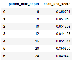
max_depths = [ 6, 8 ,10, 12, 16 ,20, 24]
# max_depth 값을 변화 시키면서 그때마다 학습과 테스트 셋에서의 예측 성능 측정
for depth in max_depths:
    dt_clf = DecisionTreeClassifier(max_depth=depth, random_state=156)
    dt_clf.fit(X_train , y_train)
    pred = dt_clf.predict(X_test)
    accuracy = accuracy_score(y_test , pred)
    print('max_depth = {0} 정확도: {1:.4f}'.format(depth , accuracy))
Decision Tree의 max_depth가 커질수록 학습 정확도가 높아지긴 하지만, 테스트 데이터 세트의 정확도는 max_depth = 8일 때 가장 높다
이는 max_depth를 너무 크게 설정하면 과적합 때문에 오히려 성능이 하락되기 때문이다
너무 복잡한 모델보다는 깊이를 낮추더라도 단순한 모델이 효과적일 수 있다
params = {
    'max_depth' : [ 8 , 12, 16 ,20],
    'min_samples_split' : [16,24],
}

grid_cv = GridSearchCV(dt_clf, param_grid=params, scoring='accuracy', cv=5, verbose=1 )
grid_cv.fit(X_train , y_train)
print('GridSearchCV 최고 평균 정확도 수치: {0:.4f}'.format(grid_cv.best_score_))
print('GridSearchCV 최적 하이퍼 파라미터:', grid_cv.best_params_)
최적 하이퍼 파라미터인 8과 몇개 값을 다시 넣어서 정확도를 확인한다
max_depth = 8, min_samples_split = 16일 때 평균 정확도 85.5% 정도로 가장 높은 수치를 나타낸다는 결과가 나왔다
best_df_clf = grid_cv.best_estimator_

pred1 = best_df_clf.predict(X_test)
accuracy = accuracy_score(y_test , pred1)
print('결정 트리 예측 정확도:{0:.4f}'.format(accuracy))
해당 파라미터를 사용하여 다시 학습한다
정확도는 87%를 기록했다
Decision Tree의 각 피처의 중요도 시각화
import seaborn as sns

ftr_importances_values = best_df_clf.feature_importances_

# Top 중요도로 정렬을 쉽게 하고, 시본(Seaborn)의 막대그래프로 쉽게 표현하기 위해 Series변환
ftr_importances = pd.Series(ftr_importances_values, index=X_train.columns  )

# 중요도값 순으로 Series를 정렬
ftr_top20 = ftr_importances.sort_values(ascending=False)[:20]
plt.figure(figsize=(8,6))
plt.title('Feature importances Top 20')
sns.barplot(x=ftr_top20 , y = ftr_top20.index)
plt.show()
seaborn을 사용하여 예측 값들이 어떤 피처에 가장 많은 영향을 받는지를 시각화한다
내림차순 정렬 후 상위 20개를 뽑는다

중요도 순으로 정렬해 보았다
위에 나온 값들이 분류에서 가장 중요한 변수들이다
여기까지 해도 아직 이 데이터 세트의 값이 무슨 동작인지 예측한 것은 아니다
참고하고 있는 파이썬 머신러닝 완벽 가이드 강의에서는 일단 여기까지 되어 있어서 결과를 도출하려면 어떻게 하는 건가 찾아봤는데 로지스틱 회귀를 써서 하는 듯 했다(data-bloom.com/notebooks/Human%20Activity%20Recognition.html#Accuracy)
회귀는 예측 이후에 나오는 내용이라 일단은 여기까지 해 두고 나중에 예측까지 해 봐야겠다
'머신러닝 > 머신러닝' 카테고리의 다른 글
| 배깅, 랜덤 포레스트 (0) | 2021.02.07 |
|---|---|
| 앙상블 개요, 보팅 (0) | 2021.02.07 |
| 분류와 결정트리, 결정트리 시각화 (0) | 2021.01.31 |
| [평가] kaggle - Pima 인디언 당뇨병 예측 (0) | 2021.01.25 |
| 평가(Evaluation)_2 (0) | 2021.01.24 |


